
Use the Excel XLOOKUP Function to Look Up Data (and Why It's Better than VLOOKUP)
by Avantix Learning Team | Updated June 27, 2026
Applies to: Microsoft® Excel® 2021, 2024 and 365 (Windows)
The XLOOKUP function is a replacement for Excel's traditional VLOOKUP function (as well as HLOOKUP and INDEX / MATCH functions). It has a new set of arguments and is available in Excel 2021, 2024 and 365. It allows you to look up a value from an array in a range or table and return one or more results. One of the primary benefits of XLOOKUP is that it can look up from columns to the left in a data set and return a range.
Contents
- Issues and limitations of VLOOKUP
- XLOOKUP with tables
- XLOOKUP function syntax
- Example 1: Basic XLOOKUP using 3 required arguments
- Example 2: XLOOKUP using error handling
- Example 3: XLOOKUP using optional error handling, match mode and search mode arguments
- Example 4: Using XLOOKUP to return data from multiple columns
- Example 5: XLOOKUP using a reverse order search
- Example 6: Advanced XLOOKUP using wildcards
- Benefits of XLOOKUP
- Issues with XLOOKUP
Recommended article: How to Lock Cells in Excel (Protect Formulas and Data)
Do you want to learn more about Excel? Check out our virtual classroom or in-person Excel courses >
Issues and limitations of VLOOKUP
XLOOKUP is most often used as an alternative to the popular VLOOKUP function to look up a value vertically in a column in a data set.
There are several issues and limitations of the VLOOKUP function:
- The VLOOKUP function looks in the first column of data for a matching value and then returns a value from a cell to the right. This is an issue if the cell you are looking up does not appear in the first column.
- You need to refer to a column number in a VLOOKUP formula (although you can work around this limitation using the MATCH function).
- VLOOKUP uses approximate match or TRUE by default.
- If you insert a new column in the data set, the VLOOKUP formula may no longer work.
- VLOOKUP returns a cell not a range.
- VLOOKUP can be slow to run on large data sets.
XLOOKUP with tables
XLOOKUP formulas can work very well with Excel tables, particularly if you add or remove columns in the table. In the table examples below, each table has been named with a tbl prefix but this is a naming convention, not a requirement. The easiest way to create a table in Excel is to select a data set (with unique field names), press Ctrl + T and click OK in the dialog box. Ensure that my table has headers is selected before clicking OK.
XLOOKUP function syntax
The XLOOKUP syntax is as follows:
=XLOOKUP(lookup_value, lookup_array, return_array, [match_mode], [search_mode])
The arguments are separated by commas. In this article, we have entered spaces after the commas for readability but typically spaces are not entered after the commas in Excel.
The first 3 arguments are required and the last arguments, which appear in square brackets, are optional.
In simple terms, the XLOOKUP syntax is as follows:
=XLOOKUP(the value you looking up, where you are looking for the value, the data you want to return or extract, is it an exact or non-exact match, how are you searching for the value)
The XLOOKUP arguments include the following:
- lookup_value (required) – the value you are searching for (which is typically a cell reference) in the lookup array. If left blank, Excel returns blank cells in the lookup array.
- lookup_array (required)– the array or range in the data set containing the lookup value (in a vertical lookup, this may be any column in the data set, does not need to be the first column, and you may refer to an entire column if the data is in an Excel table).
- return_array (required) – the array or range in the data set with the result you want to return or extract (and may be multiple columns in a data set or Excel table).
- if_not_found (optional) – the result (such as an error message) if no match is found. If nothing is entered for this argument and no match is found, #N/A will appear in the result. Text results must be entered in quotation marks for this argument (such as "No Such Customer").
- match_mode (optional) – enter 0 or FALSE for an exact match but since this is the default, this argument can be left blank. Enter 1 to return an exact match and if nothing is found, Excel will return the next larger item. Enter -1 for an exact match and if nothing is found, Excel will return the next smaller item. Enter 2 for a wildcard match with special meaning for specific characters such as *, ? and ~.
- search_mode (optional) – enter 1 to search starting from the first item and -1 to search starting from the last item. You can also enter 2 to search a lookup array sorted in ascending order and -2 to search a lookup array sorted in descending order. The results that are extracted or returned will be invalid if the array is not sorted appropriately.
Example 1: Basic XLOOKUP using 3 required arguments
In the following example, XLOOKUP is used in cell B3 to look up a value from a cell, look in a range and then a return a value from a range using the formula =XLOOKUP(B2, B7:B18, A7:A18):

Alternatively, a similar formula can be used with an Excel table. In the following example, the formula in B3 is =XLOOKUP(B2, tblEmployees[EmployeeID], tblEmployees[EmployeeName]):

In the table example, if a new column is added to the table, the XLOOKUP formula would still work. If an XLOOKUP formula is created with ranges of cells and relative referencing is used, the XLOOKUP formula may adjust if a column is added to the data.
Example 2: XLOOKUP using error handling
In the following example, the XLOOKUP formula used in the first example now includes a fourth argument to handle errors. The formula in B3 is =XLOOKUP(B2, B7:B18, A7:A18, "No such employee"):

In the table example below, a similar formula is entered. In B3, the formula is =XLOOKUP(B2, tblEmployees[EmployeeID], tblEmployees[EmployeeName], "No such employee"):

If you don't include the fourth argument, Excel will return #N/A if there is no match in the lookup array. You may use text, a number or a range for this argument.
Example 3: XLOOKUP using optional error handling, match mode and search mode arguments
In the next example, the 3 optional arguments are used:
For the if_not_found argument, 0 is entered so if there is an error or no match, 0 will be returned.
For the match_mode argument, -1 is entered so Excel will look for an exact match or the next smaller item.
For the search_mode argument, 1 is entered so Excel will search from the first item down. In this example, the data in the lookup array is sorted in ascending order.
The formula in B3 is =XLOOKUP(B2, A7:A12, B7:B12, 0, -1, 1):

In the table example below, the formula entered in B3 is =XLOOKUP(B2, tblBonus[Units Sold], tblBonus[Bonus], 0, -1, 1):

Example 4: Using XLOOKUP to return data from multiple columns
XLOOKUP can return multiple columns of data because it returns a range, not a column number. For multiple columns, the data (entered vertically) would "spill" to the right so there should not be any data entered to the right or the data cannot "spill".
In the following example, XLOOKUP is used to search for and return multiple columns of an employee's information based on their employee id. In B3, the formula is =XLOOKUP(A3, A7:A18, B7:D18, "No such employee"):

XLOOKUP will return 3 columns of data. This is a significant improvement over VLOOKUP where you need to enter multiple formulas.
In the following table example, the formula entered in B3 is =XLOOKUP(A3, tblEmployees[EmployeeID], tblEmployees[[EmployeeName]:[Sales]], "No such employee"):

Example 5: XLOOKUP using a reverse order search
You can use XLOOKUP to look for the last matching value (search in reverse order). As an example, this could be useful if you want to find the last order for a client. XLOOKUP will search from bottom to top if the lookup array is vertical and right to left if the lookup array is horizontal. In the search_mode argument, enter 1 to search first to last or -1 to search from last to first.
In the following example where the user wants to find the last order for a customer, the formula in B3 is =XLOOKUP(A3, A7:A14, B7:D14, "No such customer", 0, -1):

In the table example below, the formula in B3 is =XLOOKUP(A3, tblCustomers[CustomerID], tblCustomers[[CustomerName]:[OrderAmount]], "No such customer", 0, -1):

Example 6: Advanced XLOOKUP using wildcards
The fourth argument in XLOOKUP is match_mode and has four options:
- Enter 0 for an exact match.
- Enter 1 to return an exact match and if nothing is found, Excel will return the next larger item.
- Enter -1 for an exact match and if nothing is found, Excel will return the next smaller item.
- Enter 2 for a wildcard match with special meaning for specific characters such as *, ? and ~. This option allows partial match lookups.
The common wildcards are used as follows:
- An asterisk (*) represents any number of characters.
- A question mark (?) represents any single character.
In the following example where the user wants to be able to enter a partial name and return the employee id, the formula in B3 is =XLOOKUP("*"&A3&"*", B7:B18, A7:A18, "No such employee", 2):
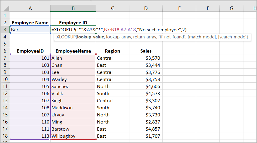
The first argument ("*"&A3&"*") allows the user to enter any characters to return a partial match so if the user entered Bar in A3, XLOOKUP would return Barstow's employee id.
In the following table example, the formula in B3 is =XLOOKUP("*"&A3&"*", tblEmployees[EmployeeName], tblEmployees[EmployeeID], "No such employee", 2):

In this example, the XLOOKUP formula will allow the use of wildcards, so the user could enter wildcards in the lookup cell. For example, in A3, the user could enter a??en to find Allen's employee id or enter bar* to find Barstow's employee id. Note that XLOOKUP is not case sensitive so you don't need to worry about entering upper case letters.
Benefits of XLOOKUP
The XLOOKUP function has many benefits:
- XLOOKUP can look left or right in a vertical data set or up or down in a horizontal data set.
- You can use only the 3 required arguments with XLOOKUP.
- XLOOKUP uses arrays so if data is added to the data set, XLOOKUP can still work.
- It can handle errors without using another function such as IFERROR.
- XLOOKUP can return an array not just a single value.
- It can make use of wildcards.
- XLOOKUP can perform reverse searches when the search_mode is -1.
Issues with XLOOKUP
XLOOKUP does have a few issues:
- You need Excel 2021 or 365 to use XLOOKUP.
- You won't be able to share workbooks using XLOOKUP with other users or clients who don't have 2021 or 365 versions of Excel.
- The arrays must be the same size.
- You can't use a column index number like VLOOKUP. You must use arrays to return values.
- If you don't refer to arrays in tables, you may need to use absolute referencing to refer to arrays.
However, for Excel users of 2021, 2024 and 365, XLOOKUP is a great new function.
Subscribe to get more articles like this one
Did you find this article helpful? If you would like to receive new articles, JOIN our email list.
More resources
How to Remove Duplicates in Excel (3 Easy Ways)
How to Convert Text to Numbers in Excel (5 Ways)
How to Merge Cells in Excel (4 Ways with Shortcuts)
How to Insert Multiple Rows in Excel (4 Fast Ways with Shortcuts)
How to Delete Blank Rows in Excel (5 Fast Ways to Remove Empty Rows)
Related courses
Microsoft Excel: Intermediate / Advanced
Microsoft Excel: Data Analysis with Functions, Dashboards and What-If Analysis Tools
Microsoft Excel: Introduction to Power Query to Get and Transform Data
Microsoft Excel: Introduction to Power Pivot and Data Models
Microsoft Excel: Introduction to Dynamic Arrays and Next-Generation Excel Functions
Microsoft Excel: Introduction to Visual Basic for Applications (VBA)
Our instructor-led courses are delivered in virtual classroom format or at our downtown Toronto location at 18 King Street East, Suite 1400, Toronto, Ontario, Canada (some in-person classroom courses may also be delivered at an alternate downtown Toronto location). Contact us at info@avantixlearning.ca if you'd like to arrange custom instructor-led virtual classroom or onsite training on a date that's convenient for you.
Copyright 2025 Avantix® Learning
You may also like

How to Replace Zeros (0) with Blanks in Excel
There are several strategies to replace zero values (0) with blanks in Excel. If you want to replace zero values in cells with blanks, you can use the Replace command or write a formula to return blanks. However, if you simply want to display blanks instead of zeros, you have two formatting options – create a custom number format or a conditional format.

What is Power Query in Excel?
Power Query in Excel is a powerful data transformation tool that allows you to import data from many different sources and then extract, clean, and transform the data. You will then be able to load the data into Excel or Power BI and perform further data analysis. With Power Query (also known as Get & Transform), you can set up a query once and then refresh it when new data is added. Power Query can import and clean millions of rows of data.

How to Freeze Rows in Excel (One or Multiple Rows)
You can freeze one or more rows in an Excel worksheet using the Freeze Panes command. If you freeze rows containing headings, the headings will appear when you scroll down. You can freeze columns as well so when you scroll to the right columns will be frozen.
Image credit(s) / application screenshot(s): Microsoft
Microsoft, the Microsoft logo, Microsoft Office and related Microsoft applications and logos are registered trademarks of Microsoft Corporation in Canada, US and other countries. All other trademarks are the property of the registered owners.
Avantix Learning |18 King Street East, Suite 1400, Toronto, Ontario, Canada M5C 1C4 | Contact us at info@avantixlearning.ca


