Use Excel Conditional Formatting to Highlight Dates Before Today (3 Ways)

Highlight Dates Before Today or Within a Date Range in Excel Using Conditional Formatting

by Avantix Learning Team | Updated October 17, 2022

Applies to: Microsoft^® Excel^® 2010, 2013, 2016, 2019, 2021 and 365 (Windows)

You can use conditional formatting in Excel to highlight cells containing dates before today or within a date range before the current date. In a worksheet, you can use conditional formatting to highlight selected cells by filling them with a color based on rules or conditions. This type of formatting is helpful if you want to highlight past due dates such as invoices that are 30, 60 or 90 days overdue.

When you apply conditional formatting, you can apply more than one rule to a range of cells.

In this article, we'll review 3 ways to highlight dates before today using conditional formatting:

1. Use built-in conditional formatting
2. Create a conditional formatting rule based on cell contents
3. Create a conditional formatting rule using a formula

Recommended article: How to Delete Blank Rows in Excel (5 Easy Ways with Shortcuts)

Do you want to learn more about Excel? Check out our virtual classroom or in-person Excel courses >

Dates must be entered or returned as valid dates in Excel in order to apply conditional formatting. Dates are affected by your regional settings and date / time settings in your Control Panel on your device.

For example, if your regional settings are set to U.S., dates are typically entered as mm/dd/yy (month / day / year) unless the date / time settings have been changed. For example, November 14, 2021 may be entered at 11/14/21 if your device's regional settings are set to U.S (you can also enter dates with dashes such as mm-dd-yy). To test your device to see how dates are recognized, press Ctrl + ; (semi-colon) in a cell in an Excel worksheet to enter the current date in the cell. Dates can then be formatted to appear in a different ways.

The current date can also be entered in a cell using the TODAY function such as =TODAY() or the NOW function such as =NOW(). The NOW function enters the current date and time whereas the TODAY function only enters the current date. They are dynamic functions so will always display the current date.

Highlight dates before today using built-in conditional formatting

To highlight dates before today using a built-in conditional formatting rule:

1. Select the cells containing dates to which you want to apply conditional formatting.
2. Click the Home tab in the Ribbon.
3. Click Conditional Formatting in the Styles group. A menu appears to the right.
4. Select Highlight Cell Rules. A menu appears.
5. From the drop-down menu, choose Dates Occurring. A dialog box appears.
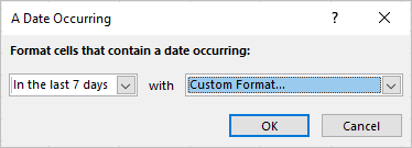
6. From the first drop-down menu, select an option such as Yesterday, In the last 7 days, Last Week, or Last Month.
7. In the second drop-down menu beside With, select Custom Format. A dialog box appears.
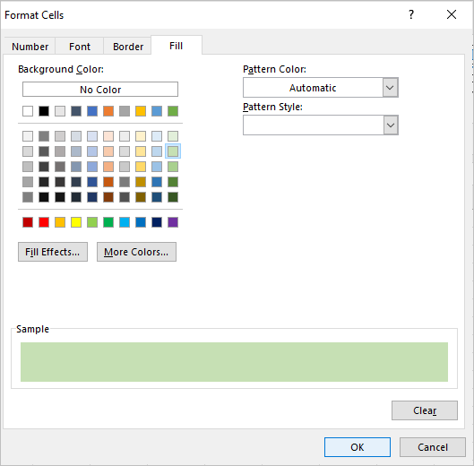
8. Click the Fill tab and then click the desired fill color. You can also click the Font tab and select a font color or another format such as bold.
9. Click OK twice.

The Date Occurring dialog box appears as follows with In the last 7 days selected (this option would include the current date):

In the Format Cells dialog box, you can select a fill as the conditional format:

Highlight dates before today by creating a conditional formatting rule based on cell contents

You can also apply your own formatting rules based on cell contents. This method gives you more control over how cells are formatted and allows you to do things you wouldn't be able to do with the built-in formats.

To highlight dates before today by creating a conditional formatting rule based on cell contents:

1. Select the cells containing dates to which you want to apply conditional formatting.
2. Click the Home tab in the Ribbon.
3. Click Conditional Formatting in the Styles group. A drop-down menu appears.
4. Select New Rule. A dialog box appears.
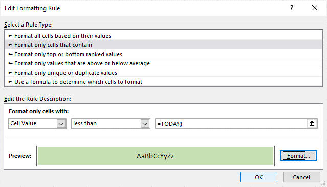
5. Select Format only cells that contain.
6. Below Format only cells with, ensure Cell Value is selected.
7. From the second drop-down menu, select less than.
8. In the text box, enter =TODAY().
9. Click Format. A dialog box appears.
10. Click the Fill tab and then click the desired fill color. You can also click the Font tab and select a font color or another format such as bold.
11. Click OK twice.

In the Edit Formatting Rule dialog box below, we entered a rule to highlight the selected cells if the cell value is less than =TODAY():

To highlight cells containing a range of dates between today and a date in the past (not including today):

1. Select the cells containing dates to which you want to apply conditional formatting.
2. Click the Home tab in the Ribbon.
3. Click Conditional Formatting in the Styles group. A drop-down menu appears.
4. Select New Rule from the drop-down menu.
5. Select Format only cells that contain.
6. Below Format only cells with, ensure Cell Value is selected.
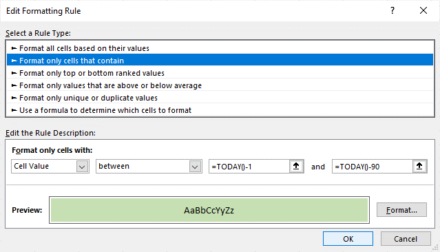
7. From the second drop-down menu, select Between.
8. In the first text box, enter =TODAY()-1.
9. In the second text box, enter another date or formula. For example, if you are looking for dates in the last 90 days before the current date, enter =TODAY()-90. For 30 days overdue, enter =TODAY()-30.
10. Click Format. A dialog box appears.
11. Click the Fill tab and then click the desired fill color. You can also click the Font tab and select a font color or another format such as bold.
12. Click OK twice.

In the Edit Formatting Rule dialog box below, we entered a rule to highlight the selected cells if the cell value is between =TODAY()-1 and =TODAY()-90 (within 90 days before the current date):

Highlight dates before today by creating a conditional formatting rule using a formula

You can use a variety of formulas in conditional formatting to change cell formats based on a formula.

When you are writing formulas in conditional formatting rules, context is very important. Write the formula as if you are in the active cell (often the first cell) and Excel, by default, uses relative referencing to copy the formula to the other cells.

To highlight dates before today by creating a conditional formatting rule using a formula:

1. Select the cells in a column containing dates to which you want to apply conditional formatting.
2. Click the Home tab in the Ribbon.
3. Click Conditional Formatting in the Styles group. A drop-down menu appears.
4. Select New Rule from the drop-down menu.
5. Click Use a formula to determine which cells to format.
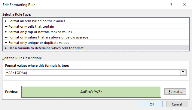
6. Enter the formula (starting with =) in the formula box (the formula references the active cell which is usually the first cell and the conditional formatting tool will adjust it for the other cells if relative referencing is used). For example, enter =A2<TODAY() if A2 is the first in the range of selected cells containing a date.
7. Click Format. A dialog box appears.
8. Click the Fill tab and then click the desired fill color. You can also click the Font tab and select a font color or another format such as bold.
9. Click OK twice.

In the Edit Formatting Rule dialog box below, we entered a formula rule of =A2<TODAY() to highlight the selected cells if the cell value is before today:

You can also use absolute and mixed referencing in conditional formatting rules.

If you want to highlight selected cells in a row with conditional formatting, select the range of cells across multiple columns and use a mixed reference with a dollar sign ($) in front of the column reference in the formula. For example, enter =$A2<TODAY() to highlight selected cells in a row before today.

Subscribe to get more articles like this one

Did you find this article helpful? If you would like to receive new articles, JOIN our email list.

More resources

How to Combine Cells in Excel Using Concatenate (3 Ways)

How to Insert Multiple Rows in Excel (4 Fast Ways with Shortcuts)

3 Excel Strikethrough Shortcuts to Cross Out Text or Values in Cells

How to Replace Blank Cells in Excel with a Value from the Cell Above

10 Excel Flash Fill Examples (Extract, Combine, Clean and Format Data with Flash Fill)

Related courses

Microsoft Excel: Intermediate / Advanced

Microsoft Excel: Data Analysis with Functions, Dashboards and What-If Analysis Tools

Microsoft Excel: Introduction to Visual Basic for Applications (VBA)

VIEW MORE COURSES >

Our instructor-led courses are delivered in virtual classroom format or at our downtown Toronto location at 18 King Street East, Suite 1400, Toronto, Ontario, Canada (some in-person classroom courses may also be delivered at an alternate downtown Toronto location). Contact us at info@avantixlearning.ca if you'd like to arrange custom instructor-led virtual classroom or onsite training on a date that's convenient for you.

Copyright 2024 Avantix^® Learning

You may also like

Microsoft, the Microsoft logo, Microsoft Office and related Microsoft applications and logos are registered trademarks of Microsoft Corporation in Canada, US and other countries. All other trademarks are the property of the registered owners.

Avantix Learning |18 King Street East, Suite 1400, Toronto, Ontario, Canada M5C 1C4 | Contact us at info@avantixlearning.ca