Turn Off or Customize Error Checking Options (and Markers) in Excel
by Avantix Learning Team | Updated September 15, 2023
Applies to: Microsoft® Excel® 2010, 2013, 2016, 2019, 2021 and 365 (Windows)
In Microsoft Excel, errors are flagged by default with a small green marker or triangle in the upper left corner of the cell. However, these indicators display when there may be an error but is, in fact, not an error. Excel checks the cells against the error checking settings or rules in the Excel Options dialog box. You can turn error checking off completely or set the rules you prefer in the Options dialog box. The default settings can cause some irritating behaviour (like flagging cells with formulas referring to empty cells).
Recommended article: 8 Tips for Entering Excel Formulas
Do you want to learn more about Excel? Check out our virtual classroom or in-person classroom Excel courses >
Change error checking options or rules
To turn off or change error checking options or rules:
- Click the File tab in the Ribbon.
- Select Options. A dialog box appears.
- Click Formulas in the left pane.
- In the right pane, select the desired options under Error Checking or Error checking rules and click OK.
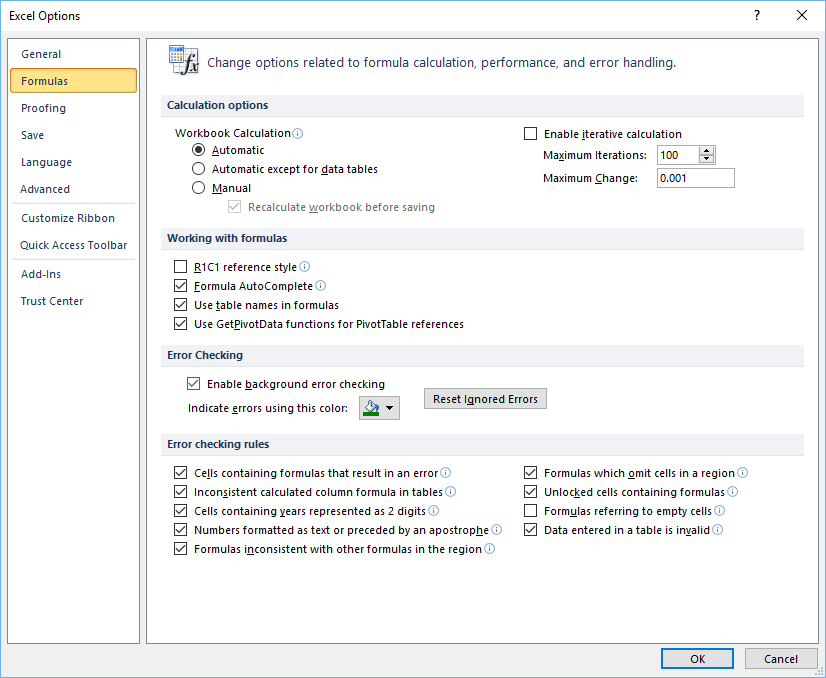
Below is the Excel Options dialog box:
Change the error marker color
To change the error marker color, in the Excel Options dialog box (Formulas category):
- Beside Indicate errors using this color, select an alternate color from the color menu.
- Click OK.
Turn off error checking
To turn off error checking completely in the the Excel Options dialog box (Formulas category):
- Deselect (uncheck) the Enable background error checking.
- Click OK.
Selecting error checking rules
You can select or deselect (check or uncheck) the following rules in the Error checking rules area in the Excel Options dialog (Formulas category):
- Cells containing formulas that result in an error – when checked, Excel displays an error indicator and adds the alert options Smart Tag to all cells that return error values.
- Inconsistent calculated column formula in tables – when checked, Excel displays an error indicator and adds the alert options Smart Tag to all cells in columns in tables that are different from other formulas in the column.
- Cells containing years represented as 2 digits – when checked, Excel displays an error indicator and adds the alert options Smart Tag to all cells that contain dates entered as text with only the last two digits of the year.
- Numbers formatted as text or preceded by an apostrophe – when checked, Excel displays an error indicator and adds the alert options Smart Tag to all cells that contain numbers entered as text (or preceded by an apostrophe).
- Formulas inconsistent with other formulas in region – when checked, Excel displays an error indicator and adds the alert options Smart Tag to all cells in which the formula is inconsistent from the others in the same area of the worksheet.
- Formulas which omit cells in a region – when checked, Excel displays an error indicator and adds the alert options Smart Tag to all cells in which a formula omits cells from the range referenced in the formula.
- Unlocked cells containing formulas – when checked, Excel displays an error indicator and adds the alert options Smart Tag to all cells containing a formula which is unlocked when the worksheet is protected.
- Formulas referring to empty cells – when checked, Excel displays an error indicator and adds the alert options Smart Tag to all cells with formulas referring to blank cells.
- Data entered in a table is invalid – when checked, Excel displays an error indicator and adds the alert options Smart Tag to all cells with formulas in which data validation has been applied and that contain values considered to be invalid.
Reset ignored errors
If a user has clicked the Smart Tag in a cell and selected Ignore Error for specific cells, this can be reset:
- In the Excel Options dialog box (Formulas category), click Reset Ignored Errors. This does not reset rules you have unchecked.
- Click OK.
Error checking markers can be very irritating and it's simple to control Excel's error checking behavior.
This article was first published on August 3, 2016 and has been updated for clarity and content.
Subscribe to get more articles like this one
Did you find this article helpful? If you would like to receive new articles, JOIN our email list.
More resources
How to Use Flash Fill in Excel (4 Ways)
How to Convert Text to Numbers in Excel (5 Ways)
How to Lock and Protect Excel Worksheets and Workbooks
10 Great Excel Navigation Shortcuts to Move Around in Workbooks
How to Replace Blank Cells in Excel with a Value from a Cell Above
Related courses
Microsoft Excel: Intermediate / Advanced
Microsoft Excel: Introduction to Power Query
Microsoft Excel: Data Analysis with Functions, Dashboards and What-If Analysis Tools
Microsoft Excel: Introduction to Visual Basic for Applications (VBA) Macros
Our instructor-led courses are delivered in virtual classroom format or at our downtown Toronto location at 18 King Street East, Suite 1400, Toronto, Ontario, Canada (some in-person classroom courses may also be delivered at an alternate downtown Toronto location). Contact us at info@avantixlearning.ca if you'd like to arrange custom instructor-led virtual classroom or onsite training on a date that's convenient for you.
Copyright 2024 Avantix® Learning
You may also like
What is Power Query in Excel?
Power Query in Excel is a powerful data transformation tool that allows you to import data from many different sources and then extract, clean, and transform the data. You will then be able to load the data into Excel or Power BI and perform further data analysis. With Power Query (also known as Get & Transform), you can set up a query once and then refresh it when new data is added. Power Query can import and clean millions of rows of data.
Excel Shortcuts to Zoom In and Out in Your Worksheets (4 Shortcuts)
There are several mouse and keyboard shortcuts you can use to zoom in and out in Excel worksheets. Some of these shortcuts are built-in and others can be created by customizing Excel Options.
How to Use Flash Fill in Excel (4 Ways with Shortcuts)
You can use Flash Fill in Excel to extract, combine, clean or format data quickly without using formulas. In order to use Flash Fill, Excel must be able to understand a pattern in a column to the left of the column where you want to fill the data so the source data should be entered in a consistent way. You can use Flash Fill by clicking a button, using shortcuts or by using the Fill handle. You run Flash Fill by entering an example of the data you want to fill using a "by example" logic.
Microsoft, the Microsoft logo, Microsoft Office and related Microsoft applications and logos are registered trademarks of Microsoft Corporation in Canada, US and other countries. All other trademarks are the property of the registered owners.
Avantix Learning |18 King Street East, Suite 1400, Toronto, Ontario, Canada M5C 1C4 | Contact us at info@avantixlearning.ca


