Insert Dynamic Screenshots Using a Camera in Microsoft Excel
by Avantix Learning Team | Updated April 7, 2021
Applies to: Microsoft® Excel® 2013, 2016, 2019 and 365 (Windows)
You can insert a live screenshot of an area in a workbook using Excel's hidden Camera. Screenshots created using this method update automatically when the original area changes. Since the Camera is a bit difficult to find, you'll need to add it to the Quick Access Toolbar (or the Ribbon) to use it.
Pictures taken with Excel's Camera are picture links (images with a formula assigned to them) which is why they will dynamically update if the original data changes. You can also use menus to take picture links.
Recommended article: How to Insert Screenshots in PowerPoint and Word
Using Camera snapshots or picture links
You can use camera snapshots or picture links in many ways including in:
- Reports or dashboards where you want to summarize data. You can use camera screenshots of key data areas or charts and resize and align them.
- Worksheets with charts where you want to see the chart change as data changes and display a smaller version of a chart.
- Workbooks where you wish to view a total from another area of your workbook.
- Shared workbooks where you want to prevent another user from changing formulas or data where you provide them with a camera snapshot that they can't change.
- Situations where you want to share a picture link with others by copying and pasting.
Adding the Camera to the Quick Access Toolbar
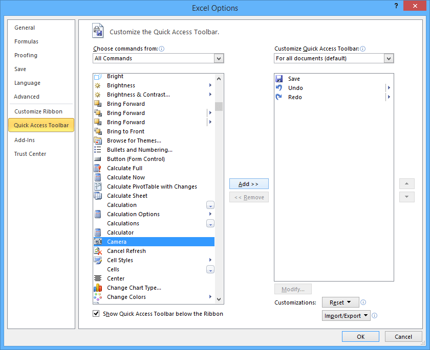
The first thing you should do is add the Camera to the Quick Access Toolbar:
- Click the File tab on the Ribbon and then click Options.
- Click the Quick Access Toolbar category on the left.
- From the drop-down menu under Choose commands from, select All Commands.
- Scroll through the list of commands and click Camera.
- Click Add.
- Click OK.
- Click Close. The Camera will appear on the Quick Access Toolbar.
The Camera appears as a button in Excel Options:
Taking a screenshot with the Camera
Note the Camera in the Quick Access Toolbar:
To take a live screenshot with the Camera:
- Select the cells you want to capture in a screenshot.
- Click on Camera on the Quick Access Toolbar. The mouse pointer will change to a cross.
- Move the mouse pointer to the location for the screenshot and drag to create a rectangle. The screenshot or picture link will be created within the box.
- Resize the picture by dragging handles that appear around the picture and align as necessary by dragging the picture (you can also use the Ribbon alignment commands). You can also apply picture effects using the Picture tab on the Ribbon when the picture is selected.
Creating picture links without using the Camera
To insert a picture link using the context menu:
- Select the cells you want to include in a live screenshot.
- Right-click and choose Copy or press Ctrl + C.
- Click where you want to insert the live screenshot.
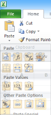
- Right-click and choose Linked Picture from the context sensitive menu or click Paste on the Home tab on the Ribbon and choose Linked Picture from the drop-down menu. Resize, align and format the picture as necessary.
Paste options appear in the Paste drop-down menu in the Ribbon:
Give it a try. It's easy to start adding picture links in Excel.
This article was first published on November 8, 2015 and has been updated for clarity and content.
Subscribe to get more articles like this one
Did you find this article helpful? If you would like to receive new articles, join our email list.
More Resources
How to Merge Cells in Excel (4 Ways with Shortcuts)
How to Combine Cells in Excel Using Concatenate (3 Ways)
3 Excel Strikethrough Shortcuts to Cross Out Text or Values in Cells
How to Highlight Errors, Blanks and Duplicates in Excel Worksheets
How to Replace Blank Cells with a Value from the Cell Above in Excel
Related courses
Microsoft Excel: Intermediate / Advanced
Microsoft Excel: Data Analysis with Functions, Dashboards and What-If Analysis Tools
Microsoft Excel: Introduction to Visual Basic for Applications (VBA)
Our instructor-led courses are delivered in virtual classroom format or at our downtown Toronto location at 18 King Street East, Suite 1400, Toronto, Ontario, Canada (some in-person classroom courses may also be delivered at an alternate downtown Toronto location). Contact us at info@avantixlearning.ca if you'd like to arrange custom instructor-led virtual classroom or onsite training on a date that's convenient for you.
Copyright 2024 Avantix® Learning
You may like
How to Replace Zeros (0) with Blanks in Excel
There are several strategies to replace zero values (0) with blanks in Excel. If you want to replace zero values in cells with blanks, you can use the Replace command or write a formula to return blanks. However, if you simply want to display blanks instead of zeros, you have two formatting options – create a custom number format or a conditional format.
What is Power Query in Excel?
Power Query in Excel is a powerful data transformation tool that allows you to import data from many different sources and then extract, clean, and transform the data. You will then be able to load the data into Excel or Power BI and perform further data analysis. With Power Query (also known as Get & Transform), you can set up a query once and then refresh it when new data is added. Power Query can import and clean millions of rows of data.
How to Freeze Rows in Excel (One or Multiple Rows)
You can freeze one or more rows in an Excel worksheet using the Freeze Panes command. If you freeze rows containing headings, the headings will appear when you scroll down. You can freeze columns as well so when you scroll to the right columns will be frozen.
Microsoft, the Microsoft logo, Microsoft Office and related Microsoft applications and logos are registered trademarks of Microsoft Corporation in Canada, US and other countries. All other trademarks are the property of the registered owners.
Avantix Learning |18 King Street East, Suite 1400, Toronto, Ontario, Canada M5C 1C4 | Contact us at info@avantixlearning.ca


