Discover the Hidden Power of Excel's Custom Views

Quickly Run Reports with Different Settings using Custom Views

by Avantix Learning | Updated May 17, 2020

Applies to: Microsoft Excel 2010, 2013, 2016, 2019 or 365 (Windows)

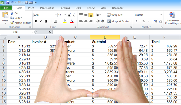
You can display several variations of the same Excel worksheet with different print settings, filters and hidden columns or rows using the powerful Custom Views command. This command is particularly useful if you are running reports for multiple audiences.

Recommended article: 10 Timesaving Excel Selection Shortcuts

What can you do with custom views?

Custom views can be used to display variations of a worksheet with different:

• Print settings including print area, margins, sheet settings and headers and footers
• Filters
• Hidden rows and columns
• Column widths and row heights
• Window settings

You can create multiple custom views in a worksheet but you can only apply a custom view to the worksheet that was active when you created the custom view.

With custom views, you could display variations of an Excel worksheet for multiple audiences such as:

• A report for managers with a set of filtered records
• A report for a client with hidden columns and filtered records
• A report for a different client with different hidden columns and different filtered records
• A default report with no filtering and no hidden columns or rows

You could also create custom views for different departments in your own organization to display data relevant to each department with different print areas.

Users can display different custom views using the Ribbon without using any VBA (Visual Basic for Applications) programming.

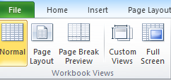
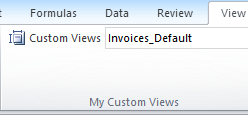
The Custom Views command appears on the View tab on the Ribbon:

Issues and limitations

Custom views have a few limitations:

• They cannot be used in a workbook where named tables (not pivot tables) have been created (using Insert Table or Format as Table).
• Users may not be able to access custom views if protection has been applied in a worksheet used in a custom view.

Creating a default custom view

It's a good idea to create a default custom view first with the settings you use most often. This could be a default view with no hidden columns or rows and no filtering.

To create a default custom view:

1. Set up the worksheet with the print settings, filtering and hidden rows and/or columns you prefer.
2. Click the View tab in the Ribbon.
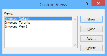
3. Click Custom Views. The Custom Views dialog box appears.
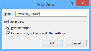
4. Click Add.
5. Enter a name for the view such as Invoices_Default. You may use spaces. It's a good idea to include the name of the worksheet as well.
6. Check the options you wish to include in the view.
7. Click OK.

Creating alternate custom views

Once you have created the default custom view, you can create multiple alternate views:

1. Set up the worksheet with the print settings, filtering and hidden rows and/or columns for the view.
2. Click the View tab in the Ribbon.
3. Click Custom Views. The Custom Views dialog box appears.
4. Click Add.
5. Enter a name for the view such as Invoices_View1 or Invoices_Toronto.
6. Check the options you wish to include in the view.
7. Click OK.
8. Repeat the process for any other views.

Adding a drop-down list of views by customizing the Ribbon

To make it easy to display different custom views, you can add a drop-down list of custom views to the Ribbon:

1. Click the File tab in the Ribbon.
2. Click Options.
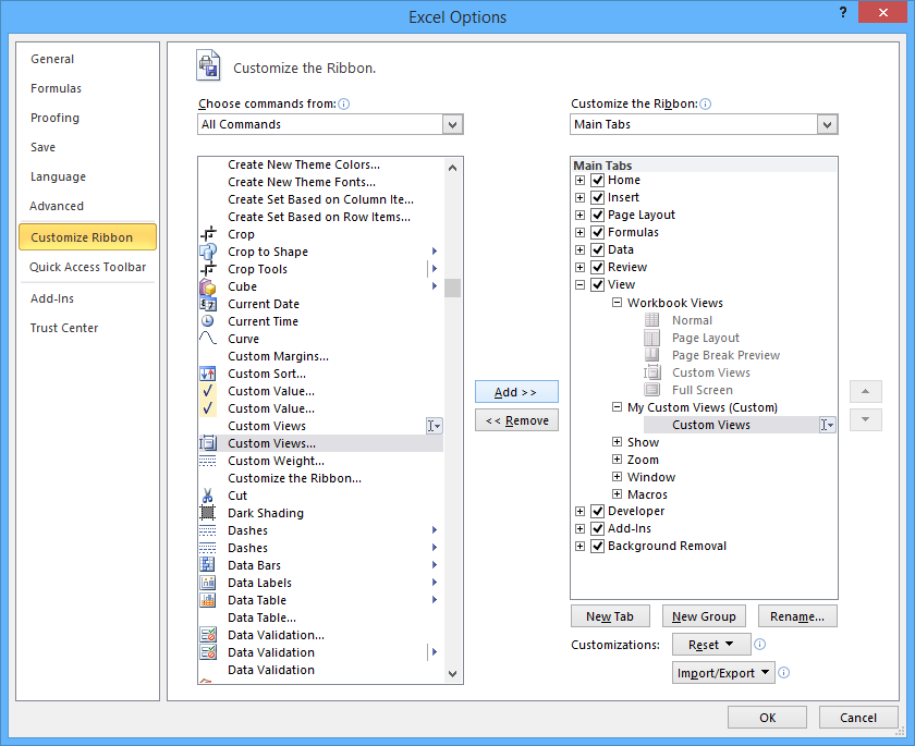
3. In the categories on the left, click Customize Ribbon.
4. On the right side of the window, click on the plus sign (+) to the left of the View tab.
5. Click Workbook Views to select that Group and then click the New Group button.
6. With the New Group selected, click Rename.
7. Type a name for the new group and click OK. For example, enter My Custom Views.
8. With the My Custom Views group selected, click on the drop-down arrow for Choose Commands From.
9. Select Commands Not in the Ribbon under Choose Commands from.
10. Scroll down and click Custom Views and then click Add to move that command to the My Custom Views group.
11. Click OK.

Displaying custom views

To display custom views if you have not customized the Ribbon:

1. Click the View tab in the Ribbon.
2. Click Custom Views.
3. Click the view you wish to apply.
4. Click Show.

To display different custom views if you have customized the Ribbon and added a drop-down menu:

1. Click the View tab in the Ribbon.
2. Select a custom view from the Custom Views drop-down list you added if you customized the Ribbon.

Editing a custom view

To edit a custom view:

1. Apply the custom view.
2. Make any changes to the filters, layout and print settings in the worksheet.
3. Create a new custom view and name it the same name as the one you want to replace.
4. Click OK. A dialog appears.
5. Click Yes to replace the old custom view with the current view.

Deleting a custom view

To delete a custom view:

1. Click the View tab in the Ribbon.
2. Click Custom Views.
3. Click the View you wish to delete.
4. Click Delete. A dialog box appears.
5. Click Yes to delete the view.

Custom views are another one of those overlooked tools that can save you a lot of time in Excel.

Subscribe to get more articles like this one

Did you find this article helpful? If you would like to receive new articles, join our email list.

More resources

How to Merge Cells in Excel (with Shortcuts)

How to Use Flash Fill in Excel (4 Ways with Shortcuts)

How to Insert or Type Greek Letters or Symbols in Excel (6 Ways)

10 Great Excel Navigation Shortcuts to Move Around is Your Workbooks

How to Change Commas to Decimal Points in Excel and Vice Versa (5 Ways)

Related courses

Microsoft Excel: Intermediate / Advanced

Microsoft Excel: Data Analysis with Functions, Dashboards and What-If Analysis Tools

Microsoft Excel: Introduction to Power Query to Get and Transform Data

Microsoft Excel:  Visual Basic for Applications (VBA) | Introduction

VIEW MORE COURSES >

Our instructor-led courses are delivered in virtual classroom format or at our downtown Toronto location at 18 King Street East, Suite 1400, Toronto, Ontario, Canada (some in-person classroom courses may also be delivered at an alternate downtown Toronto location). Contact us at info@avantixlearning.ca if you'd like to arrange custom instructor-led virtual classroom or onsite training on a date that's convenient for you.

Copyright 2024 Avantix^® Learning

You may also like

Microsoft, the Microsoft logo, Microsoft Office and related Microsoft applications and logos are registered trademarks of Microsoft Corporation in Canada, US and other countries. All other trademarks are the property of the registered owners.

Avantix Learning |18 King Street East, Suite 1400, Toronto, Ontario, Canada M5C 1C4 | Contact us at info@avantixlearning.ca