
How to Quickly Select Columns, Rows and Ranges in Excel Tables
by Avantix Learning Team | Updated March 21, 2024
Applies to: Microsoft® Excel® 2016, 2019, 2021 and 365 (Windows)
There are many different shortcuts for selecting elements in Microsoft Excel tables. You can use shortcuts to select an entire table, an entire row, an entire column or ranges in tables.
Keep in mind that a table in Excel is created by converting a data set to a table. It is not simply data entered in columns and rows. Tables are one of Excel's most important tools and a table is, essentially, a dynamic named range.
Recommended article: 10 Great Pivot Table Shortcuts
Do you want to learn more about Excel? Check out our virtual classroom or in-person classroom Excel courses >
Data that is going to be converted into an Excel table should:
- Be entered in columns and rows with column headings in the first row and similar data entered in the rows below
- Have unique column headings
- Have no merged cells
It's also a good idea to remove blank columns and blank rows.
You can convert a data set to a table in 3 ways:
- Click in the data set and then click the Home tab in the Ribbon. Click Format as Table in the Styles group and click a style in the gallery. In the dialog box that appears, ensure My table has headers is checked and click OK.
- Click in the data set and then click the Insert tab in the Ribbon. Click Table in the Tables group. In the dialog box that appears, ensure My table has headers is checked and click OK.
- Click in the data set and then press Ctrl + T. In the dialog box that appears, ensure My table has headers is checked and click OK.
Once your data set has been converted to a table, you can use the following shortcuts.
1. Select a table using a mouse
To select a table, move your mouse over the top left corner of the table until a diagonal arrow appears:
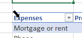
Click the top left corner of the table once to select the table data.
Click the top left corner of the table twice to select the table including the table headers.
2. Select a table using a keyboard
To select an entire table, select any cell in the table and press Ctrl + A to select the table data.
To select an entire table including the header row, select any cell in the table and then press Ctrl + A twice.
You can also select the first cell of the table and then press Ctrl + Shift + right arrow and then press Ctrl + Shift + down arrow.
3. Select a column using a mouse
To select a column in a table, move the cursor to the top of a table column header until a down arrow appears:
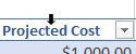
Click the top edge of the table column header once to select the table column data.
Click the top edge of the table column header twice to select the entire table column including the header.
4. Select a column using a keyboard
To select a column, select any cell in a table column and press Ctrl + Spacebar to select the table column data.
Press Ctrl + Spacebar twice to select the table column data and header.
You can also select the first cell in the table column and then press Ctrl + Shift + down arrow.
5. Select a row or rows using a mouse
To select a row in a table, move the cursor to the left border of the table row until a right-pointing arrow appears:
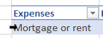
Click to select the current row or drag up to down to select multiple rows.
You can also click the first cell in the table row and then press Ctrl + Shift + right arrow to select the row.
6. Select rows using a mouse and keyboard
To select multiple contiguous rows, move the cursor to the left border of the first row of the table until it changes into a right-pointing selection arrow and then click to select the row. Press Shift and click with the selection arrow on the last row you want to select.
To select multiple non-contiguous rows, move the cursor to the left border of the first table row until it changes into a right-pointing selection arrow and then click to select the row. Press Ctrl and click with the selection arrow on subsequent rows.
7. Select a row or rows using a keyboard
To select a row in a table, select any cell in the row and press Shift + Spacebar once.
You can also select the first cell in a row and press Ctrl + Shift + right arrow.
If you want to select rows below the selected row, press Shift + down arrow.
Subscribe to get more articles like this one
Did you find this article helpful? If you would like to receive new articles, JOIN our email list.
More resources
How to Remove Duplicates in Excel (3 Easy Ways)
How to Lock Cells in Excel (Protect Formulas and Data)
How to Fill Blank Cells in Excel with a Value from a Cell Above
How to Combine Cells in Excel Using CONCATENATE (3 Ways)
How to Insert Multiple Rows in Excel (4 Fast Ways with Shortcuts)
Related courses
Microsoft Excel: Intermediate / Advanced
Microsoft Excel: Data Analysis with Functions, Dashboards and What-If Analysis Tools
Microsoft Excel: Introduction to Visual Basic for Applications (VBA)
Our instructor-led courses are delivered in virtual classroom format or at our downtown Toronto location at 18 King Street East, Suite 1400, Toronto, Ontario, Canada (some in-person classroom courses may also be delivered at an alternate downtown Toronto location). Contact us at info@avantixlearning.ca if you'd like to arrange custom instructor-led virtual classroom or onsite training on a date that's convenient for you.
Copyright 2024 Avantix® Learning
You may also like

How to Replace Zeros (0) with Blanks in Excel
There are several strategies to replace zero values (0) with blanks in Excel. If you want to replace zero values in cells with blanks, you can use the Replace command or write a formula to return blanks. However, if you simply want to display blanks instead of zeros, you have two formatting options – create a custom number format or a conditional format.

What is Power Query in Excel?
Power Query in Excel is a powerful data transformation tool that allows you to import data from many different sources and then extract, clean, and transform the data. You will then be able to load the data into Excel or Power BI and perform further data analysis. With Power Query (also known as Get & Transform), you can set up a query once and then refresh it when new data is added. Power Query can import and clean millions of rows of data.

How to Freeze Rows in Excel (One or Multiple Rows)
You can freeze one or more rows in an Excel worksheet using the Freeze Panes command. If you freeze rows containing headings, the headings will appear when you scroll down. You can freeze columns as well so when you scroll to the right columns will be frozen.
Microsoft, the Microsoft logo, Microsoft Office and related Microsoft applications and logos are registered trademarks of Microsoft Corporation in Canada, US and other countries. All other trademarks are the property of the registered owners.
Avantix Learning |18 King Street East, Suite 1400, Toronto, Ontario, Canada M5C 1C4 | Contact us at info@avantixlearning.ca