Excel Shortcuts for Filtering Data (10+ Keyboard Shortcuts)

How to Filter or AutoFilter Excel Data Quickly using Keyboard Shortcuts

by Avantix Learning Team | Updated April 17, 2023

Applies to: Microsoft^® Excel^® 2013, 2016, 2019, 2021 and 365 (Windows)

You can turn on Filter or AutoFilter in Excel for data sets / lists and tables and easily filter and sort data using a mouse or keyboard shortcuts. When you first turn on Filter, arrows appear in the header row for each field with a drop-down menu. You can use keyboard shortcuts to select different filter options from the Filter menus or remove the filters.

Note that filter options change depending on the type of data in the column – text, numbers, dates or times.

You can create three types of filters or autofilters – by value(s), by criteria or by a format (such as a color). Depending on the filter you apply, you may need to clear one filter before applying another filter.

Do you want to learn more about Excel? Check out our instructor-led virtual classroom or in-person classroom Excel courses >

The following are 10 useful keyboard shortcuts to filter data in Excel.

1. Turn Filter / AutoFilter on

To turn Filter on using a keyboard shortcut, ensure a cell in the range is selected and then press Ctrl + Shift + L. If your data range contains any blank columns or rows, select the entire range of cells first. You can use the same shortcut to turn the Filter off.

Down arrows will appear beside field names in the header row as follows:

If you have converted a list to a table, the Filter arrows should automatically appear.

2. Display the Filter menu

To use a shortcut to display the Filter menu for a column:

Select a cell in the header row that contains a Filter arrow.
Press Alt + down arrow to display the Filter menu for the column.

3. Select Filter menu options using shortcuts

Once the Filter menu is displayed by pressing Alt + down arrow, you can use shortcuts including your arrow keys to navigate the menu and press Enter and the Spacebar to select and apply filters:

Press the up or down arrow keys to select a command
Press Enter to apply the command
Press the Spacebar to check or uncheck a checkbox

4. Clear or remove all filters

To clear or remove all filters for all fields in the current filtered range, select a cell in the range and press Alt > A > C. This is a sequential shortcut so press Alt then A and then C. Do not press Shift. This is a key tip shortcut that accesses the Ribbon.

You can also press Ctrl + Shift + L to turn Filter off which will remove the filters. Press Ctrl + Shift + L to turn Filter on again.

5. Clear or remove filters in a column

To clear or remove the filters in a column:

Select a cell in the header row and press Alt + down arrow to display the Filter menu for the column.
Type the letter C to clear the filter.

6. Filter by typing underlined characters

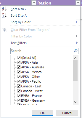
Once the Filter menu is displayed, you can type underlined letters to select a filter option. The underlined letters that appear in the menu are the shortcut keys for each command. For example, typing the letter F would display the Text, Number or Date Filters sub-menu. Do not press Shift while typing these characters.

Note the underlined characters in the menu below:

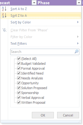
7. Sort by typing underlined characters

Once the Filter menu is displayed, you can type characters to sort (do not hold down Shift) as follows:

Type S to sort in ascending order
Type O to sort in descending order
Type T to sort by color (then select the color you want using your arrow keys and press Enter)

8. Filter using the Search box

To use the Search box to filter:

Select a cell in the header row and press Alt + down arrow to display the Filter menu for the selected column.
Type the letter E to jump to the Search box where you can type your criteria.

Note the Search box in the menu below:

9. Display the Custom Filter dialog box

When you want to filter using custom criteria, you can display the Custom Filter / AutoFilter dialog box:

Select a cell in the header row and press Alt + down arrow to display the Filter menu for the column.
Type the letter F.
Type the letter E (this displays the Custom Filter dialog box which sets the comparison operator to Equal).
Select options from the menus (such as Equal, Not Equal, etc.) and enter criteria.
Select And or Or.
Press Enter to apply the filter.

Enter criteria in criteria boxes in the Custom Filter / AutoFilter dialog box below:

In the Custom Filter dialog box, you can keep pressing Tab to select different options in the dialog.

10. Filter blanks or non-blanks

To filter to display blank cells in the selected column:

Select a cell in the header row and press Alt + down arrow to display the Filter menu for the column.
Type the letter F.
Type the letter E (this displays the Custom Filter dialog box which sets the comparison operator to Equal).
Press Enter.

To filter to display non-blank cells in the selected column:

Select a cell in the header row and press Alt + down arrow to display the Filter menu for the column.
Type the letter F.
Type the letter N (this displays the Custom Filter dialog box which sets the comparison operator to Does Not Equal).
Press Enter.

11. Filter to display top values

To filter to display top values in the selected column containing numbers:

Select a cell in the header row and press Alt + down arrow to display the Filter menu for the column.
Type the letter F.
Type the letter T (a dialog box appears).
Enter the number of top items you want (such as 3).
Press Enter.

If you use filters a lot, these keyboard shortcuts can save you quite a bit of time.

This article was first published on January 23, 2017 and has been updated for clarity and content.

Subscribe to get more articles like this one

Did you find this article helpful? If you would like to receive new articles, JOIN our email list.

More resources

How to Freeze Row and Column Headings in Excel Worksheets

3 Excel Strikethrough Shortcuts to Cross Out Text or Values in Cells

How to Highlight Errors, Blanks and Duplicates in Excel Worksheets

How to Replace Blank Cells in Excel with Zeros (0), Dashes (-) or Other Values

10 Excel Flash Fill Examples (Extract, Combine, Clean and Format Data with Flash Fill)

Microsoft Excel: Data Analysis with Functions, Dashboards and What-If Analysis Tools

Microsoft Excel: Introduction to Visual Basic for Applications (VBA)

VIEW MORE COURSES >

Our instructor-led courses are delivered in virtual classroom format or at our downtown Toronto location at 18 King Street East, Suite 1400, Toronto, Ontario, Canada (some in-person classroom courses may also be delivered at an alternate downtown Toronto location). Contact us at info@avantixlearning.ca if you'd like to arrange custom instructor-led virtual classroom or onsite training on a date that's convenient for you.

What is Power Query in Excel?

Power Query in Excel is a powerful data transformation tool that allows you to import data from many different sources and then extract, clean, and transform the data. You will then be able to load the data into Excel or Power BI and perform further data analysis. With Power Query (also known as Get & Transform), you can set up a query once and then refresh it when new data is added. Power Query can import and clean millions of rows of data.

How to Stop or Control Green Error Checking Markers in Excel

In Microsoft Excel, errors are flagged with small green marker or triangle in the upper left corner of the cell. However, these indicators display when there may be an error but is, in fact, not an error.

Excel Shortcuts to Zoom In and Out in Your Worksheets (4 Shortcuts)

There are several mouse and keyboard shortcuts you can use to zoom in and out in Excel worksheets. Some of these shortcuts are built-in and others can be created by customizing Excel Options.

Excel Shortcuts for Filtering Data (10+ Keyboard Shortcuts)