
10 Useful Tips for Summarizing Data Using Excel's Subtotal Feature
by Avantix Learning Team | Updated April 9, 2021
Applies to: Microsoft® Excel® 2010, 2013, 2016, 2019 and 365 (Windows)
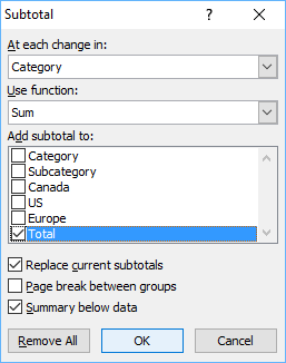
You can insert subtotals in Microsoft Excel data sets or lists using the Subtotal feature (which appears on the Data tab in the Ribbon) to summarize data.
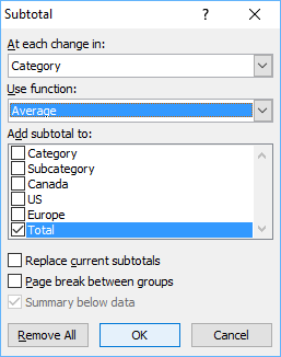
Below is the Subtotal dialog box:
Recommended article: No Mouse? Using Keyboard Only Navigation in Microsoft Office (Part 1: The Ribbon)
Do you want to learn more about Excel? Check out our virtual classroom or live classroom Excel courses >
Check out the following tips when working with the Subtotals feature in Microsoft Excel.
1. You can't use the Subtotal feature with Excel tables
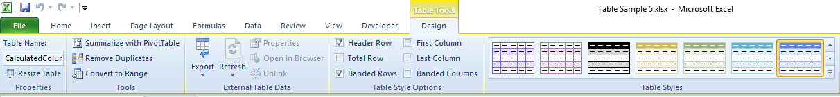
If your data is an Excel table (created using the Table feature on the Insert tab or the Format tab in the Ribbon), you can't use the Subtotals feature. To see if you data set is a table, click in the data and take a look at the Ribbon. If you see Table Tools Design or Table Design in the Ribbon, your data set is an Excel table.
Below is the Table Tools Design tab in the Ribbon:
2. Clean up your data set
Data sets should be set up correctly with unique column headings or field names in the first row, no merged cells and no blank rows or blank columns within the data set.
In order to use the Subtotal feature effectively, the data set must be clean or consistent. For example, if you have city data with Toronto spelled as Toronto, Tornto or Tononto, you would get 3 different subtotals. It's best to clean up these types of inconsistencies first before inserting subtotals.
3. Always sort first and then add subtotals
Always sort your data set first and then subtotal by the first sort key. So if you want to subtotal by city, sort by city first and then add subtotals at each change in city.
4. Collapse or expand the outline
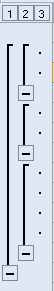
When you insert subtotals using the Subtotal feature, Excel applies an outline and an outline pane appears on the left of the worksheet. You can click the numbers on the top left to display different levels in the outline (also called collapsing or expanding the outline).
If you insert subtotals once, Excel creates three levels in the outline, but Excel can display up to eight levels.
The levels show the following if you insert one set of subtotals:
- 1 displays grand totals
- 2 displays subtotals and grand totals
- 3 displays data, subtotals and grand totals
Below is the outline pane with 3 levels:
5. Remove subtotals when you no longer need them
You can remove subtotals at any time. Simply click in the data set (or the header row), click the Data tab in the Ribbon, click Subtotals in the Outline group and then click Remove All.
Below is the Subtotal dialog box (note the Remove All button at the bottom):
6. Show or hide the outline pane
You can show or hide the outline pane by pressing Ctrl + 8.
The outline pane will be removed automatically if you remove subtotals.
7. Apply multiple subtotal functions
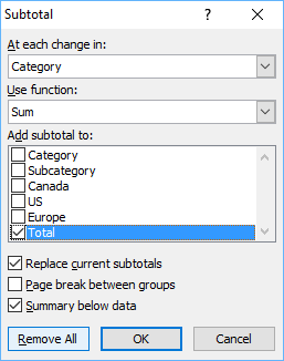
You can apply multiple subtotal functions in your data set. For example, you may want to calculate the sum, average and number of orders for each product. In order to do this, you would need to sort by product and then insert subtotals 3 times and uncheck the Replace Current Subtotals option in the Subtotal dialog box.
Below is the Subtotal dialog box with Replace Current Subtotals unchecked:
8. Format subtotals and grand totals
It can be tricky to format subtotals and grand totals as users often accidentally format the data set or records as well.
To format only subtotals and grand totals:
- Click the appropriate number in the outline pane to display subtotals and grand totals.
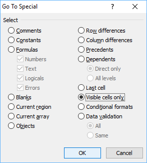
- Select only visible cells by pressing Alt + ; (semi-colon). Alternatively, press Control + G to display the Go To dialog box, click Special to display the Go to Special dialog box, click Visible Cells Only and then click OK.
- Apply the desired formats such as bold or a cell style.
- Click the appropriate number in the outline pane to display all data.
Below is the Go to Special dialog box:
9. Remove unwanted labels in subtotals
When you insert subtotals, Excel adds labels such as Total, Average and Count in the subtotal row.
To remove the labels, you can use Excel's Find and Replace as follows:
- Click the column (such as column B) with the labels you want to replace.
- Press Ctrl + H. The Find and Replace dialog box appears.
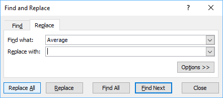
- Enter the label you wish to find (such as Average) in the Find What box.
- Ensure there is nothing entered in the Replace With box.
- Click Replace All or click Replace and then Find Next to go through each subtotal.
- Click OK and then click Close.
Below is the Find and Replace dialog box:
10. Copy subtotals and grand totals to another worksheet
If you collapse the outline and then try to copy only the subtotals and grand totals to another worksheet or workbook, Excel will copy the data set, the subtotals and grand totals by default.
To copy only the subtotals and grand totals:
- Click the appropriate number in the outline pane to collapse the outline and display only subtotals and grand totals. If you do not want to include grand totals, select the rows with the subtotals by selecting the row headings.
- Select only visible cells by pressing Alt + ; (semi-colon). Alternatively, press Ctrl + G to display the Go To dialog box, click Special to display the Go to Special dialog box, click Visible Cells Only and then click OK.
- Press Ctrl + C to copy the visible cells to the Clipboard.
- Click in a target cell (such as A1) in a new worksheet.
- Press Ctrl + V to paste the cells. The visible cells will be copied down and to the right of the target cell.
The Subtotal feature is very useful for summarizing data in Excel. These tips will help you get the results you want.
This article was first published on September 9, 2018 and has been updated for clarity and content.
Subscribe to get more articles like this one
Did you find this article helpful? If you would like to receive new articles, join our email list.
More resources
How to Fill Blank Cells in Excel with a Value from a Cell Above
How to Use Flash Fill in Excel to Clean or Extract Data (Beginner's Guide)
How to Quickly Delete Blank Rows in Excel (5 Ways)
Related courses
Microsoft Excel: Intermediate / Advanced
Microsoft Excel: Data Analysis with Functions, Dashboards and What-If Analysis Tools
Microsoft Excel: Introduction to Visual Basic for Applications (VBA)
Our instructor-led courses are delivered in virtual classroom format or at our downtown Toronto location at 18 King Street East, Suite 1400, Toronto, Ontario, Canada (some in-person classroom courses may also be delivered at an alternate downtown Toronto location). Contact us at info@avantixlearning.ca if you'd like to arrange custom instructor-led virtual classroom or onsite training on a date that's convenient for you.
Copyright 2024 Avantix® Learning
You may also like

How to Replace Zeros (0) with Blanks in Excel
There are several strategies to replace zero values (0) with blanks in Excel. If you want to replace zero values in cells with blanks, you can use the Replace command or write a formula to return blanks. However, if you simply want to display blanks instead of zeros, you have two formatting options – create a custom number format or a conditional format.

What is Power Query in Excel?
Power Query in Excel is a powerful data transformation tool that allows you to import data from many different sources and then extract, clean, and transform the data. You will then be able to load the data into Excel or Power BI and perform further data analysis. With Power Query (also known as Get & Transform), you can set up a query once and then refresh it when new data is added. Power Query can import and clean millions of rows of data.

How to Freeze Rows in Excel (One or Multiple Rows)
You can freeze one or more rows in an Excel worksheet using the Freeze Panes command. If you freeze rows containing headings, the headings will appear when you scroll down. You can freeze columns as well so when you scroll to the right columns will be frozen.
Microsoft, the Microsoft logo, Microsoft Office and related Microsoft applications and logos are registered trademarks of Microsoft Corporation in Canada, US and other countries. All other trademarks are the property of the registered owners.
Avantix Learning |18 King Street East, Suite 1400, Toronto, Ontario, Canada M5C 1C4 | Contact us at info@avantixlearning.ca